• 01 Overview
• 02 Linear Algebra
• 03~04 Transformation
  • 1. 2D Transformation
    • 1.1 Affine Transformation
    • 1.2 Homogenous Coordinates
    • Affine Transformation in Homogeneous Coordinates
    • Example: Rotating Around a Given Point
  • 2. 3D Transformation
  • 3. Viewing Transformation
    • 3.1 View Transformation
    • 3.2 Projection Transformation
      • 3.2.1 Orthographic Projection
      • 3.2.2 Perspective Projection
• $$ M_{\text{persp} \to \text{ortho}} \begin{bmatrix} x \ y \ z \ 1 \end{bmatrix}
• \begin{bmatrix} nx/z \ ny/z \ \text{unknown} \ 1 \end{bmatrix}
• $$ M_{\text{persp} \to \text{ortho}} \begin{bmatrix} x \ y \ n \ 1 \end{bmatrix}
• \begin{bmatrix} x \ y \ n \ 1 \end{bmatrix}
• $$ M_{\text{persp} \to \text{ortho}} \begin{bmatrix} 0 \ 0 \ f \ 1 \end{bmatrix}
• 05~06 Rasterization
  • 1. Defining the screen space
  • 2. Viewport Transformation
  • 3. Rasterization
  • 4. Sampling Artifacts
    • Explaination
  • 5. Anti-aliasing
    • MSAA
• 07~09 Shading
  • 8. Texture Magnification/Minification
    • 8.1 Texture Magnification
    • 8.2 Texture Minification
• 10~12 Geometry
• 13~16 Ray Tracing
  • 1. Recursive (Whitted-Style) Ray Tracing
    • 1.1 Ray-Surface Intersection
      • 1.1.1 Ray Equation
    • Ray Definition
      • 1.1.2 Ray Intersection With Implicit Surface
      • 1.1.3 Ray Intersection With Triangle
    • 1.2 Accelerating Ray-Surface Intersection
    • 1.2.1 Bounding Volume
  • 2. Using AABBs to Accelerate Ray Tracing
    • 2.1 Uniform Grid
    • 2.2 Spatial Partition
    • 2.3 Object Partition & Bounding Volume Hierarchy (BVH)

GAMES101：现代计算机图形学入门，是GAMES(Graphics And Mixed Environment Symposium)组织开设的一门线上课。讲师是闫令琪，现在是加州大学圣芭芭拉分校助理教授。我在去年九月末两周时间刷完了GAMES101（共22节课），并做了一波整理。虽然这两周经历了一些小麻烦，但是还是顺利做完了这份整理。

01 Overview

The course content mainly includes:

• Rasterization: Displaying geometric shapes in 3D space on the screen. Real-time rendering (30fps) is a significant challenge.
• Geometry Representation: How to represent curves, surfaces, and topological structures.
• Ray Tracing: Slow but realistic. Achieving real-time performance is a major challenge.
• Animation/Simulation: For example, when throwing a ball to the ground, how it bounces, compresses, and deforms.

02 Linear Algebra

Be confident, you know it all!

• Dot Product: Can determine front and back, as shown in the diagram below.
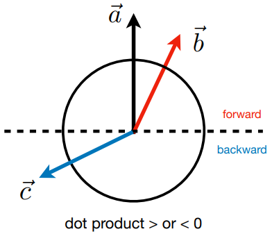
• Cross Product: It can determine left and right, as well as inside and outside, as shown in the diagram below.
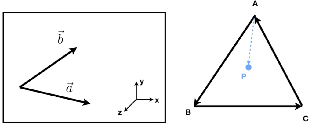
  • Left Diagram: Determine left and right by checking the sign of the cross product result.
  • Right Diagram: Determine whether a point is inside or outside a triangle by checking if it lies on the same side of all three edges.

03~04 Transformation

1. 2D Transformation

1.1 Affine Transformation

Affine transformation consists of linear transformation and translation.

The transformation formula is:

where the first term is a linear transformation, and the second term is translation.

The corresponding linear transformation matrix $\begin{bmatrix} a & b \\ c & d \end{bmatrix}$ is:

• Scaling (scale):

  $s_{\alpha, \beta} = \begin{bmatrix} \alpha & 0 \\ 0 & \beta \end{bmatrix}$

  The reference position is the origin. The x-axis scales by a factor of α, and the y-axis scales by a factor of β.

• Shear (shear): $\begin{bmatrix} 1 & a \\ 0 & 1 \end{bmatrix}$

  The reference position is the origin. The vertical coordinates of all points remain unchanged, while the horizontal coordinates shift.

• Rotation (rotate): $R_{\theta} = \begin{bmatrix} \cos\theta & -\sin\theta \\ \sin\theta & \cos\theta \end{bmatrix}$ A counterclockwise rotation by an angle θ around the origin. The rotation matrix is an orthogonal matrix, meaning: $R_{\theta}^T = R_{\theta}^{-1}$ The rotation matrix derivation can be easily obtained using the transformations: $(1,0) \rightarrow (\cos\theta, \sin\theta), \quad (0,1) \rightarrow (-\sin\theta, \cos\theta)$

1.2 Homogenous Coordinates

Previously, we saw the affine transformation equation:

However, handling translation terms can be cumbersome. By introducing homogeneous coordinates, we can elegantly incorporate translations. The concept of homogeneous coordinates is to represent an $n$-dimensional coordinate using an $n+1$-dimensional vector.

For 2D transformations, we use 3D vectors to represent 2D coordinates (adding a $w$-axis alongside $x$ and $y$):

• 2D point: $(x, y, 1)^T$
• 2D vector: $(x, y, 0)^T$
• Extended homogeneous form: $(x, y, w)$ where $w \neq 0$ is equivalent to $(x/w, y/w, 1)^T$.

Regarding the $w$-axis, a point's homogeneous coordinate typically has $w = 1$, while a vector has $w = 0$. This makes sense because adding a vector to a vector results in a vector, adding a point to a point is not defined, and adding a vector to a point results in a point.

Affine Transformation in Homogeneous Coordinates

Affine transformations can be rewritten as (typically performing linear transformation first, then translation):

Example: Rotating Around a Given Point

Let's look at an example of how to rotate around a given point in a unified way:

1. $T(-c)$: Translate to the origin
2. $R(\alpha)$: Rotate by angle $\alpha$
3. $T(c)$: Translate back to the original point

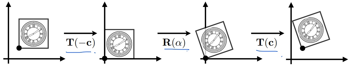
The entire process can be written as:

2. 3D Transformation

Similarly, homogeneous coordinates can be used to represent:

• 3D point = $(x, y, z, 1)^T$
• 3D vector = $(x, y, z, 0)^T$
• $(x, y, z, w)^T$ ($w \neq 0$) is extended to be equivalent to $(x/w, y/w, z/w, 1)^T$

Affine transformations can be written as (still applying the linear transformation first, then translation):

Components:

• Scaling:

  $$S(s_x, s_y, s_z) = \begin{bmatrix} s_x & 0 & 0 & 0 \\ 0 & s_y & 0 & 0 \\ 0 & 0 & s_z & 0 \\ 0 & 0 & 0 & 1 \end{bmatrix}$$

• Translation:

  $$T(t_x, t_y, t_z) = \begin{bmatrix} 1 & 0 & 0 & t_x \\ 0 & 1 & 0 & t_y \\ 0 & 0 & 1 & t_z \\ 0 & 0 & 0 & 1 \end{bmatrix}$$

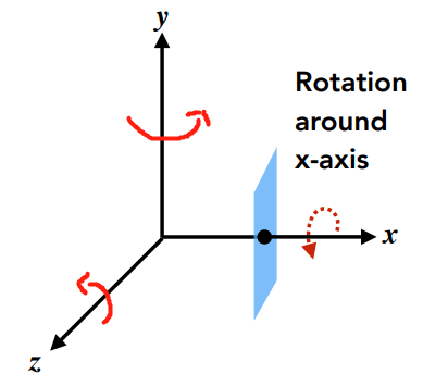
• Rotation around the x-, y-, and z-axes:

  • Rotation about the x-axis:

    $$R_x(\alpha) = \begin{bmatrix} 1 & 0 & 0 & 0 \\ 0 & \cos \alpha & -\sin \alpha & 0 \\ 0 & \sin \alpha & \cos \alpha & 0 \\ 0 & 0 & 0 & 1 \end{bmatrix}$$

  • Rotation about the y-axis:

    $$R_y(\alpha) = \begin{bmatrix} \cos \alpha & 0 & \sin \alpha & 0 \\ 0 & 1 & 0 & 0 \\ -\sin \alpha & 0 & \cos \alpha & 0 \\ 0 & 0 & 0 & 1 \end{bmatrix}$$

  • Rotation about the z-axis:

    $$R_z(\alpha) = \begin{bmatrix} \cos \alpha & -\sin \alpha & 0 & 0 \\ \sin \alpha & \cos \alpha & 0 & 0 \\ 0 & 0 & 1 & 0 \\ 0 & 0 & 0 & 1 \end{bmatrix}$$

The positive direction of rotation is as shown in the figure. The derivation process is similar to the 2D rotation case.

3D rotation can be decomposed into sequential rotations about the x-, y-, and z-axes:

where $\alpha, \beta, \gamma$ are known as Euler angles.

Rodrigues' Rotation Formula

In 3D space, a vector $\mathbf{v}$ rotating around an arbitrary axis $\mathbf{n} = (n_x, n_y, n_z)$ by an angle $\alpha$ results in the transformed vector $\mathbf{R}(\mathbf{n}, \alpha) \mathbf{v}$. The corresponding rotation matrix is given by:

where $\mathbf{I}$ is the identity matrix.

Proof Omitted

3. Viewing Transformation

viewing transformation

• view transformation or camera transformation
• projection transformation
  • orthographic projection
  • perspective projection

3.1 View Transformation

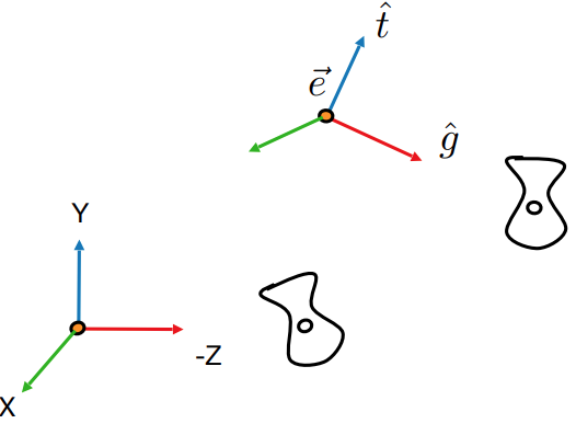Understanding these parameters is analogous to adjusting the rotation of a photograph. We assume $\mathbf{g} \perp \mathbf{t}$, but the camera's upward direction is conventionally defined by humans. Establishing an orthonormal basis can help avoid distortions during view transformations.

If we maintain the relative positions of the camera and objects while translating both, the objects appear unchanged to the camera. Naturally, we want to move the camera to a fixed position, commonly known as the look-at point, where the look-at direction $\mathbf{g}$ aligns with the negative z-axis, and the up direction $\mathbf{t}$ corresponds to the y-axis.

This process is called view transformation or camera transformation, denoted as $M_{\text{view}}$. Specifically:

First, we perform the translation transformation, where $\mathbf{e} = (x_e, y_e, z_e)$, and subscripts like $\mathbf{t}$ and $\mathbf{g}$ follow similar notation:

Next, we apply the rotation transformation, aligning $\mathbf{g}$, $\mathbf{t}$, and $\hat{\mathbf{g}} \times \mathbf{t}$ with the negative z-axis, y-axis, and x-axis, respectively. The inverse rotation matrix $R_{\text{view}}^{-1}$ is given by:

Since rotation matrices are orthogonal, we obtain:

By substituting these into the equation, we obtain the camera transformation $M_{\text{view}}$.

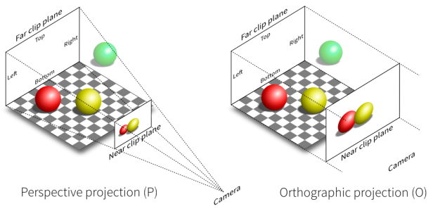
3.2 Projection Transformation

Now that the camera and objects are positioned correctly, the objects need to be projected from 3D to a 2D plane. There are two types of projection:

• Orthographic projection
• Perspective projection

However, the projection transformation introduced below actually maps a cuboid into a $[-1,1]^3$ space.

3.2.1 Orthographic Projection

Simplified Understanding of Orthographic Projection:

• The camera is at the origin, looking along the negative z-axis, with the up direction aligned with the y-axis.
• Drop off the z-axis.
• The object is translated and scaled into the range $[-1,1]^2$, meaning both the x- and y-coordinates are confined between $-1$ and $1$.

Common Approach:

Consider a cuboid defined by the ranges $[l, r] \times [b, t] \times [f, n]$. This cuboid is transformed into the canonical cube $[-1,1]^3$, which means:

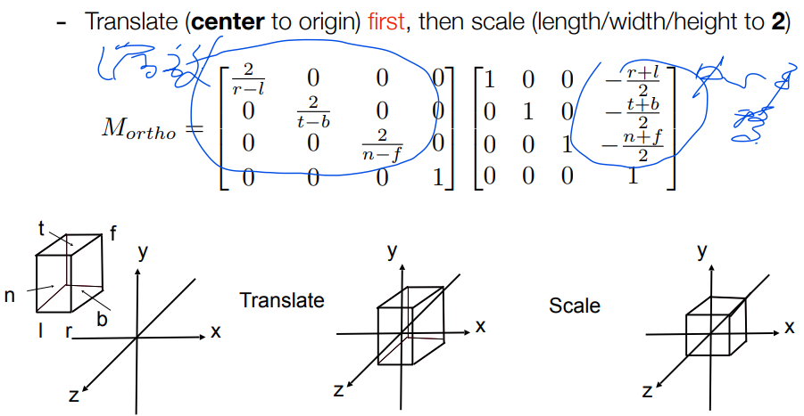When using a right-handed coordinate system:

• The left side has a smaller x value than the right.
• The bottom has a smaller y value than the top.
• However, the front has a larger z value than the back.

This is why OpenGL uses a left-handed coordinate system, where the depth axis (z) is more intuitive for rendering.

3.2.2 Perspective Projection

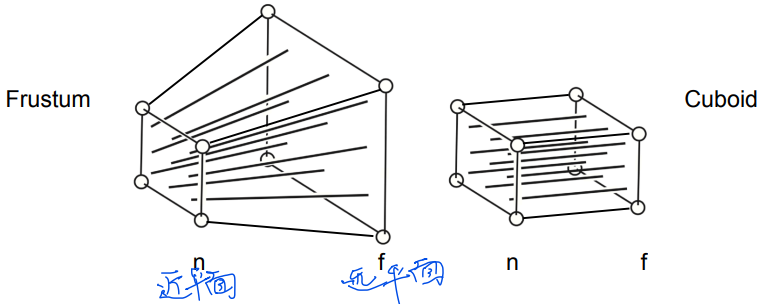Steps for Perspective Projection:

• $M_{\text{persp} \to \text{ortho}}$: Transforms the frustum into a cuboid by "squeezing" it, ensuring that any point on the near plane remains unchanged, the z-coordinate on the far plane remains unchanged. while modifying the z-coordinates of intermediate planes.

• $M_{\text{ortho}}$: Applies orthographic projection, as discussed in section 3.2.1.

• Finally, the perspective projection matrix is:

  $$M_{\text{persp}} = M_{\text{ortho}} M_{\text{persp} \to \text{ortho}}$$

  which gives the final result.

Derivation of $M_{\text{persp} \to \text{ortho}}$

Consider an arbitrary point $(x, y, z)$ in the frustum. After transformation by $M_{\text{persp} \to \text{ortho}}$, it is scaled into the form $(nx/z, ny/z, \text{unknown})$ (which follows from similar triangles):

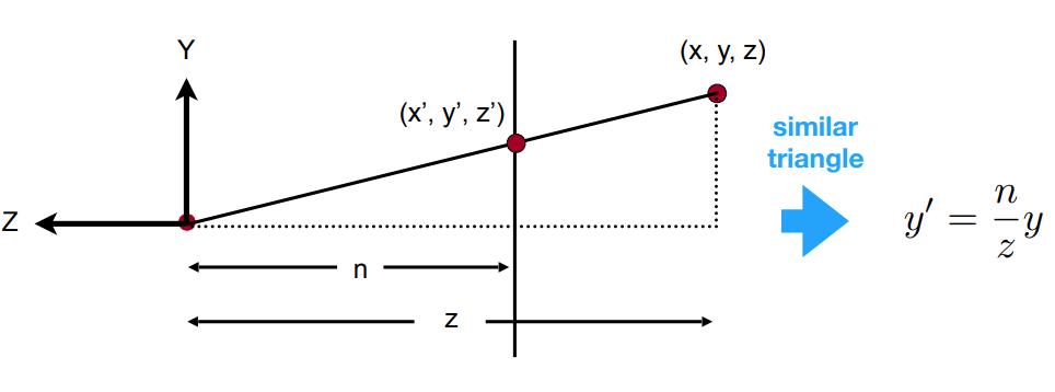
Thus, the transformation matrix $M_{\text{persp} \to \text{ortho}}$ takes the form:

Since a point on the near plane remains unchanged and the z-coordinate on the far plane is preserved, we have:

Solution:

From this, we derive the perspective-to-orthographic transformation matrix:

Computing $l, r, b, t$ Using $fov_Y$ and Aspect Ratio

Previously, the near plane was defined using:

• $l$ (x-coordinate of the left edge),
• $r$ (x-coordinate of the right edge),
• $b$ (y-coordinate of the bottom edge),
• $t$ (y-coordinate of the top edge).

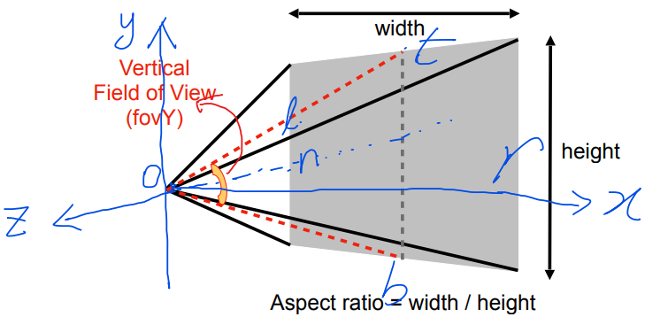Alternatively, we can express these parameters using the vertical field of view (field-of-view, $fov_Y$) and the aspect ratio (width-to-height ratio). Clearly, we have:

• $t = |n| \tan \frac{fov_Y}{2}$
• $r = t \cdot aspect$
• $b = -t, \quad k = -r$

05~06 Rasterization

After the projection transformation, the object has been translated and scaled into the $[-1,1]^3$ space.

Now, to render the object onto the screen, we perform rasterization.

1. Defining the screen space

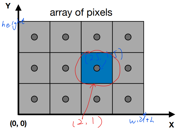
• Screen range: $(0,0)$ to $(\text{width}, \text{height})$
• Pixels are represented by integers $(x, y)$, e.g., the pixel at $(2,1)$ in the red circle.
• Pixel range: $(0,0)$ to $(\text{width}-1, \text{height}-1)$
• The center of a pixel $(x, y)$ is located at $(x + 0.5, y + 0.5)$.

2. Viewport Transformation

Given that the object has already been translated and scaled into the $[-1,1]^3$ space, we now want to translate and scale it into the screen range $[0, \text{width}] \times [0, \text{height}]$, while discarding the z-axis.

This process is known as the viewport transformation

The transformation matrix is straightforward to derive:

3. Rasterization

A triangle mesh is a widely used and effective method for representing objects. The advantages of choosing triangles include:

• The most fundamental polygon: Any other polygon can be decomposed into triangles.
• Always planar: A triangle is always a flat surface.
• Well-defined inside and outside: It has a clear distinction between the interior and exterior.
• Good interpolation properties: Enables smooth gradients and shading effects.

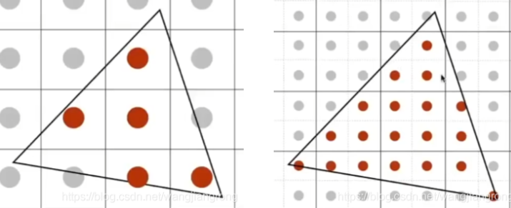
How to Represent a Triangle Using Pixels?

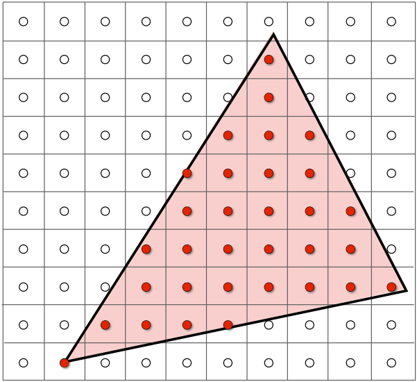
The approach is to sample and check whether each pixel center lies inside the triangle.

for (int x = 0; x < xmax; x++)
    for (int y = 0; y < ymax; y++)
        image[x][y] = inside(tri, x + 0.5, y + 0.5);
        // inside function: returns 1 if inside the triangle, otherwise 0

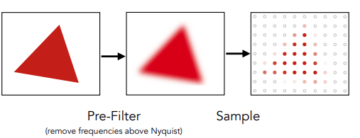
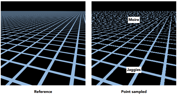
4. Sampling Artifacts

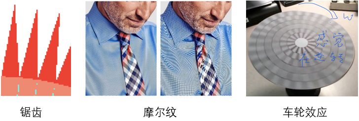
Common sampling artifacts include:

• Jaggies (锯齿):
  Caused by insufficient resolution, leading to visible stair-step edges on diagonal lines.

• Moire Pattern (摩尔纹):
  Occurs when sampling frequency is too low relative to the image details.
  Example: Removing odd-numbered rows/columns from an image and reconstructing it.

• Wagon Wheel Effect (车轮效应):
  An illusion where wheels appear to rotate backward due to mismatched frame rates and object movement.

• Other Artifacts:

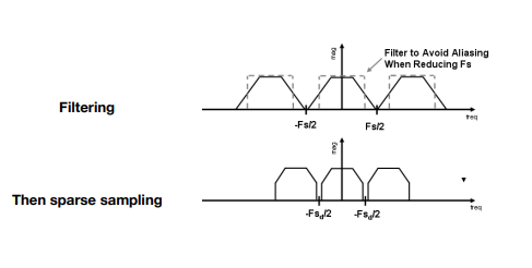
Sampling artifacts are also known as aliasing.
This occurs when the signal changes too quickly, but the sampling rate is too low, leading to distortions.

Explaination

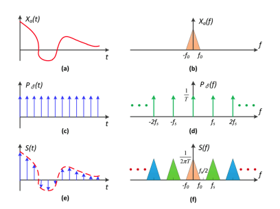Sampling = Repeating Frequency Contents Aliasing = Mixed Frequency Contents

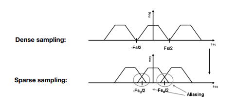
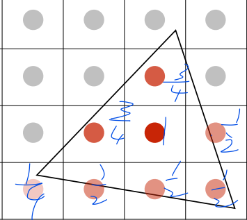
5. Anti-aliasing

Filtering out high frequencies before sampling (Blurring) Before Sampling

MSAA

MSAA is an approximation of the first step of blurring.

07~09 Shading

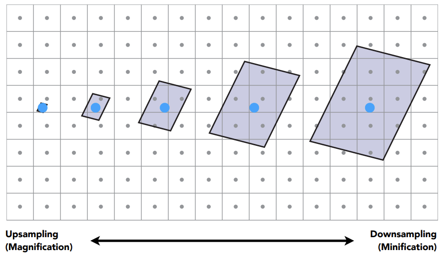
8. Texture Magnification/Minification

When applying textures, several issues may arise:

• Texture Magnification:

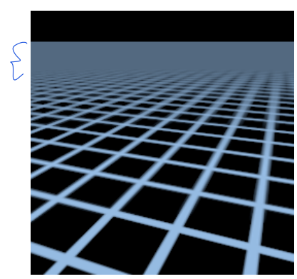
  • Occurs when the texture resolution is too low.
  • Multiple screen pixels map to the same (u,v) coordinate, leading to blocky artifacts.
  • This results in unnatural transitions at boundaries, forming visible pixelated grids (see Figure 8.1, Nearest).

• Texture Minification:

  • Occurs when the texture resolution is too high.
  • A single pixel on the screen maps to multiple (u,v) coordinates.
  • This causes aliasing artifacts, as fine texture details cannot be properly represented (see Figure 8.2).

8.1 Texture Magnification

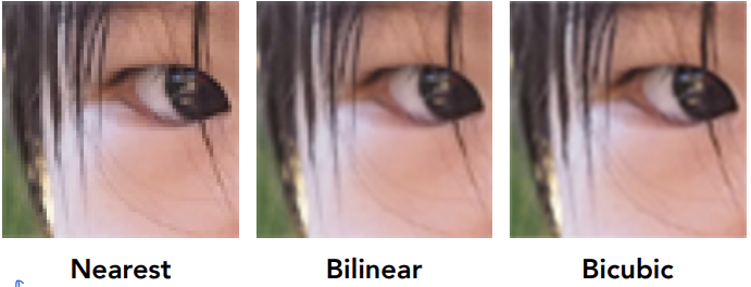Three Approaches to Texture Mapping Nearest Neighbor Filtering: Simply selects the nearest texel for each pixel. Fast but produces blocky artifacts, especially when magnified.

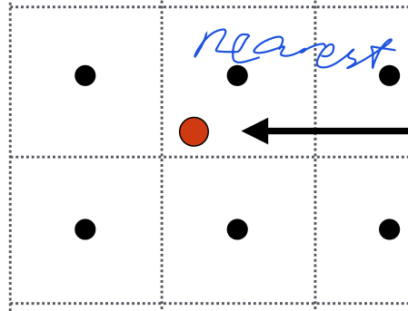
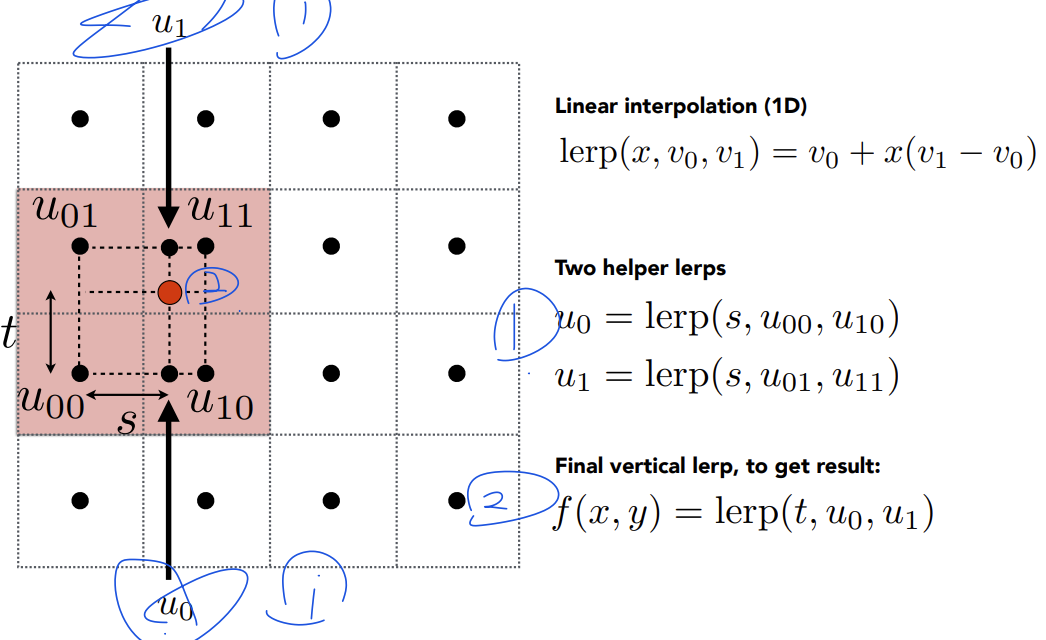
Bilinear Filtering:

• Selects the four nearest texels.
• Performs two passes of linear interpolation to compute the final color.

8.2 Texture Minification

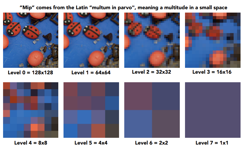
Supersampling can be used to solve aliasing issues, but it is computationally expensive. The following introduces the concept of Mipmap, which allows fast, approximate, and square-shaped range queries—providing an immediate average (or maximum, minimum, etc.) value within a region.

Using the original texture, a mipmap is generated through preprocessing. The additional storage required is only one-third of the original image, making it efficient in terms of memory usage.

Screen pixels only need to sample the corresponding level of texels. But how do we compute the level $D$?

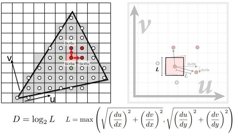Below is an approximate method: (Refer to 3Blue1Brown’s explanation of the Jacobian matrix for more details.) Suppose we calculate a level of 1.8. Trilinear interpolation is required to obtain the final value for the screen pixel, which involves performing two bilinear interpolations followed by a linear interpolation.

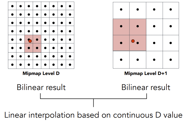
However, since mipmaps only perform range queries within square regions, an overblur issue arises. When a screen pixel corresponds to a rectangular or even diagonally elongated region in the texture, the mipmap naturally selects a larger square for sampling, leading to unintended blurring. To address this issue, anisotropic filtering and EWA filtering can be used. These methods generate different texture maps that support range queries beyond just square regions.

10~12 Geometry

13~16 Ray Tracing

1. Recursive (Whitted-Style) Ray Tracing

Let's first learn about a traditional ray tracing algorithm known as Whitted-style ray tracing.

This method differs from conventional shading models in several key ways:

• Light Interaction: Unlike standard shading, this method assumes that light rays continue to reflect and refract after hitting an object.
• Shading Process: Each time reflection or refraction occurs (a bounce point), shading is computed, provided the point is not in shadow.

As shown in the diagram, this recursive process allows for realistic effects such as reflections, refractions, and shadows.

1. Cast a ray from the viewpoint through the image plane and check for intersections with objects.
2. Generate reflection and refraction rays upon intersection.
3. Recursively trace the generated rays to compute lighting effects.
4. Each bounce point is shaded based on its visibility to the light source.
5. Combine all shading contributions using weighted summation to determine the final pixel color.

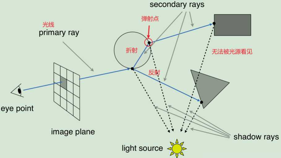To facilitate further explanations, the course defines the following concepts:

• Primary Ray: The initial ray cast from the viewpoint that first intersects an object.
• Secondary Rays: Rays generated after bouncing off a surface, including reflection and refraction rays.
• Shadow Rays: Rays used to determine visibility between a point and a light source.

1.1 Ray-Surface Intersection

1.1.1 Ray Equation

Ray Definition

A ray can be defined by a point o and a direction vector d as:

1.1.2 Ray Intersection With Implicit Surface

As illustrated in the diagram:

• Ray equation:

  $$r(t) = o + t d, \quad 0 \leq t < \infty$$

• General implicit surface:

  $$p: f(p) = 0$$

• Substituting the ray equation:

  $$f(o + t d) = 0$$

• Solve for real, positive roots to determine intersection points.

1.1.3 Ray Intersection With Triangle

Calculation Steps:

1. Find the intersection between the ray and the plane containing the triangle.
2. Check whether the intersection point lies inside the triangle.

Finding the Ray-Plane Intersection

Moller Trumbore Alogrithm A fast method to determine whether a ray intersects a triangle and to compute the intersection point relies on barycentric coordinates to represent the plane.

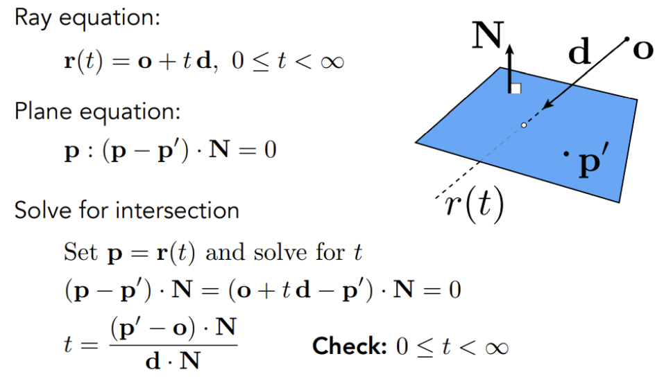
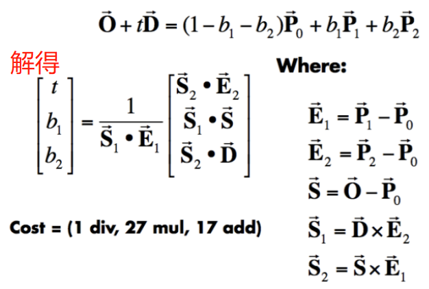
• Solve for $t$, $b_1$, and $b_2$ using three equations with three unknowns.
• Check validity of the solution:
  • The intersection must be along the ray direction ($t \geq 0$).
  • The intersection point must be inside the triangle ($b_1 \geq 0$, $b_2 \geq 0$).

1.2 Accelerating Ray-Surface Intersection

Instead of checking for intersections between the ray and every triangle, we first check if the ray intersects a bounding box that encloses the object.

• If the ray does not intersect the bounding volume, it definitely does not intersect the object.
• If the ray does intersect the bounding volume, then we proceed with a more detailed intersection test.

1.2.1 Bounding Volume

One commonly used bounding volume is the Axis-Aligned Bounding Box (AABB).

• An AABB is aligned with the coordinate axes, meaning its faces are parallel to the xOy, yOz, or zOx planes.
• During intersection testing, checking against an AABB first helps eliminate unnecessary intersection tests with complex geometry.
• If the ray intersects the AABB, we proceed with a more precise intersection test with the actual object.

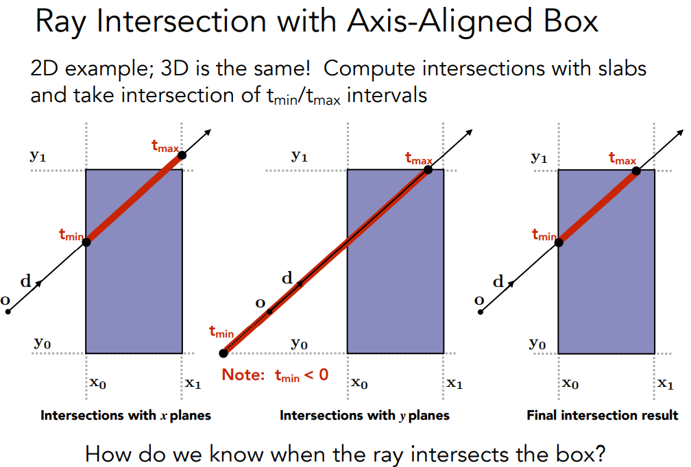
Key Concepts for Ray-AABB Intersection

1. The ray enters all slabs (pairs of parallel planes) before it is considered inside the bounding box.
2. If the ray exits any slab, it is considered to have left the bounding box.
3. An intersection occurs when $t_{\text{enter}} < t_{\text{exit}}$.
4. If $t_{\text{exit}} < 0$, the box is behind the ray, meaning there is no valid intersection.
5. If $t_{\text{exit}} \geq 0$ and $t_{\text{enter}} \leq 0$, the ray starts inside the box and intersects it.
6. For a 3D bounding box, the entry and exit times are computed as:
   • $t_{\text{enter}} = \max(t_{\min})$
   • $t_{\text{exit}} = \min(t_{\max})$

Conclusion: A ray intersects the AABB if and only if $t_{\text{enter}} \leq t_{\text{exit}}$ and $t_{\text{exit}} \geq 0$.

(This algorithm is based on the Liang-Barsky algorithm.)

2. Using AABBs to Accelerate Ray Tracing

2.1 Uniform Grid

2.2 Spatial Partition

2.3 Object Partition & Bounding Volume Hierarchy (BVH)